How to Analyze the Performance of a Kalman Filter Generated from MATLAB?

Today, I’ll walk you through a step-by-step performance analysis of a well-known signal processing filter: a Kalman filter generated in C from MATLAB.

To do that, I’ll be using beLow-Explore, our product to analyze the performance debt in a C/C++ software.

You can find the chosen use-case here. You’ll probably think it is a very small use-case and you’ll get it right! But think about it, if you can detect a performance debt on hundreds of lines of code what you could detect in bigger projects?

Let’s jump right into the analysis process!

This article presents how to analyze the performance debt of a C generated source code from MATLAB and demonstrates that several ways for performance improvement are detected and could bring up to 45% gain in execution time.

It explains how auditing your source code with a good combination of static and dynamic analysis as well as checking a list of points of caution can improve software performance and understanding of the behavior of your application.

Here’s exactly how we are doing on this concrete example.

• First, from the generated source code of the filter, we are creating a bench to execute the filter on a set of representative input data. This first step will allow us to get dynamic information on the filter.
• Then, we are configuring the project with the filter and the bench to execute it in the product beLow-Explore. By launching the analysis on the project, we’ll be able to gather varied comprehensive metrics to understand where we are spending time in our filter. A checklist of several optimization techniques (remember the points of caution?) will be run through to check if parts of the source code should be rewritten / modified so as to solve performance debt points and improve the software execution speed.
• The result? In less than a minute, the analysis can indicate to you whether your code has no or little optimization potential for performance (Yaaay 🎉) or if your code has points to be improved so as to gain in execution time. In this particular example, we improved the execution time of the filter by 45%.

1 – Create your test bench

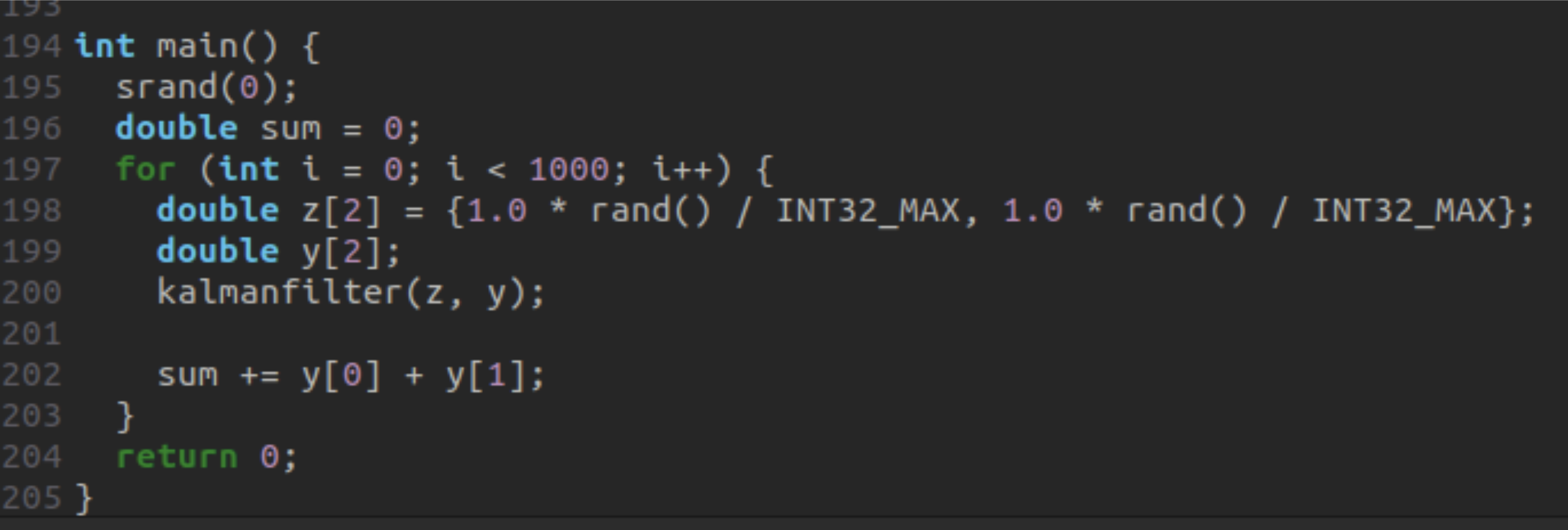
Start by creating your test bench to execute your filter on a set of representative input data. For the generated Kalman filter, we want to analyze the function called kalmanfilter() from the file kalmanfilter.c, taking as inputs two values represented with double data-types.

We will generate input data to feed this function. It looks like this (no science in it, just for demonstration 😉):

You now have a folder containing your Kalman filter C source code (taken from MATLAB), the main function to execute the filter on the representative input data, and in our case a Makefile to build the project (we’ll use gcc 11.4 to build in O2; if you are using another compiler and want to know more about our technical compatibility). This folder will be imported into beLow-Explore to launch the analysis. Remember that the analysis done by beLow is dependent on a hardware target that will execute the piece of code to analyze? To keep it simple, we’ll take our computer in this case (Ref. Intel i7 1255U). Note that it can be any CPU supported by beLow.

Want to know more about this or about digital signal processors compatibility?

2 – Run the analysis in beLow-Explore

Since we have chosen to do the analysis on the function kalmanfilter(), this function and its callee will be analyzed. We’ll then get a dashboard with the analysis metrics.

For instance, let’s focus on the complexity information:

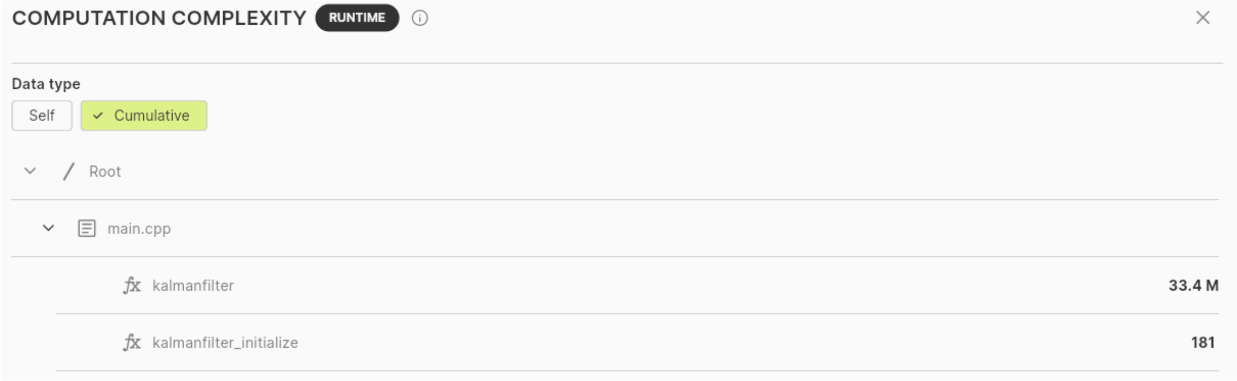
We can see that there are very few functions in the code and that the initialization function kalmanfilter_initialize() has very little influence on the global complexity (which seems rather logical). Therefore, our focus will be on the main function: the one and only, kalmanfilter().

If we want to jump more on what composes this complexity, let’s check the “functionality repartition” information:

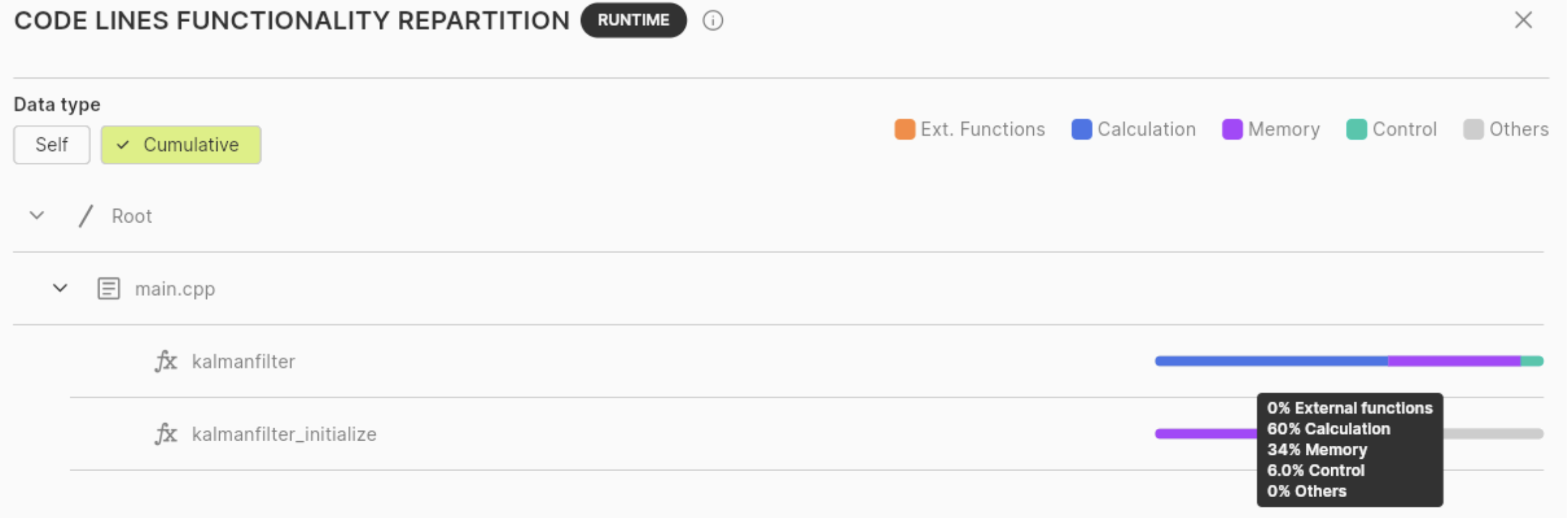
We can see that the kalmanfilter() function spends the majority of its time (60%) in calculation (add, multiply, division… operations). Almost the rest of the time (34%) is spent in memory operations (load, store operations). If we want to reduce the execution time of this function, we’ll then have to focus on  the computation part.

3 – Evaluate performance improvement potential

To end with, we’ll determine if this function has no potential for performance improvement or if our caution points are flashing red. Given the information provided by the dashboard below, we can see that we have a potential to reduce the execution time by 45% (in CPU cycles).

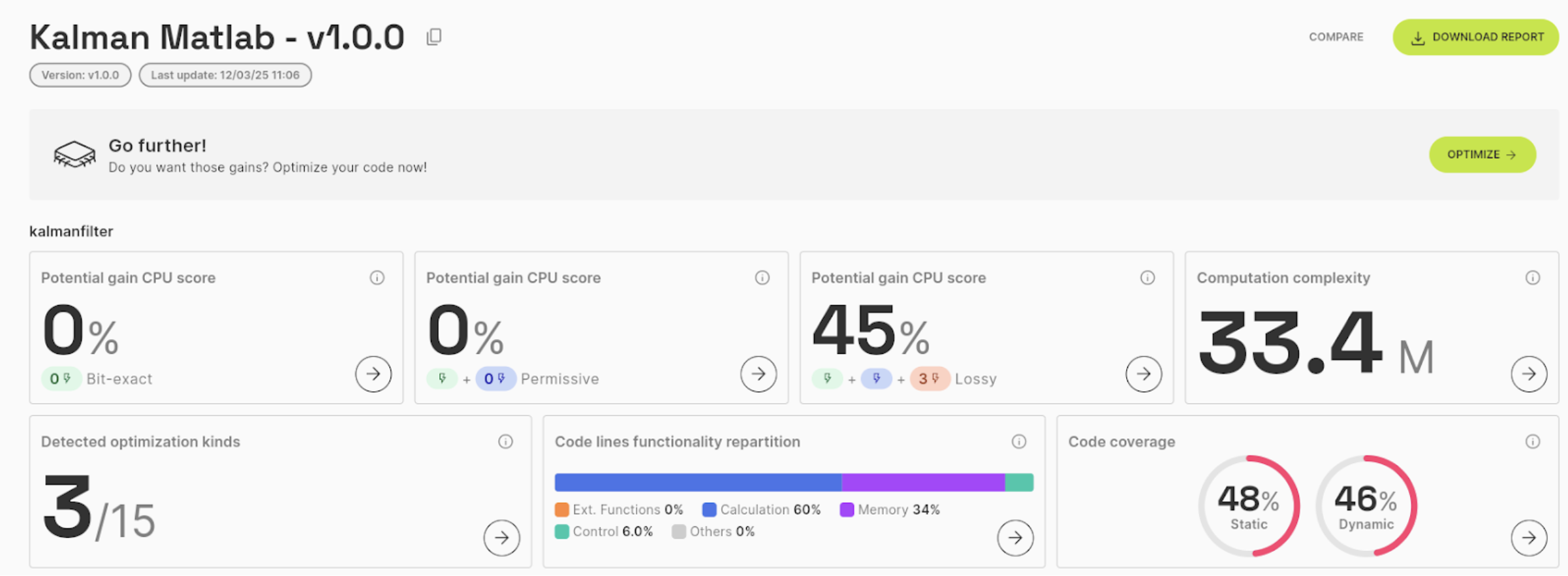
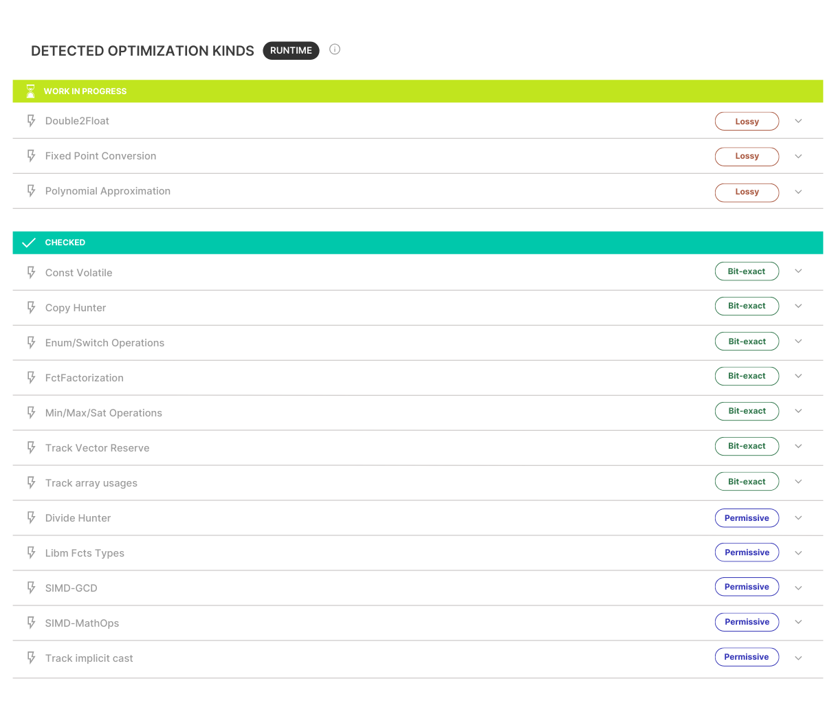
On the checklist of caution points, we can see below (and not beLow 😉) that 12 caution points have been tested with success in this code, which is already very good! 3 caution points remain to rework (data-types and polynomial approximation in this case) and could bring up to 45% of reduction in execution time.

If you follow this process to regularly analyze the performance of your software applications, you’ll probably quickly reach an optimization potential to zero and improve your product performance as well as your development time!

Hoping this article helped, again, do not hesitate to give any feedback on it or on any additional deep dive you’d like to see!

		Justine Bonnot CEO & Founder of WedoLow Let’s connect